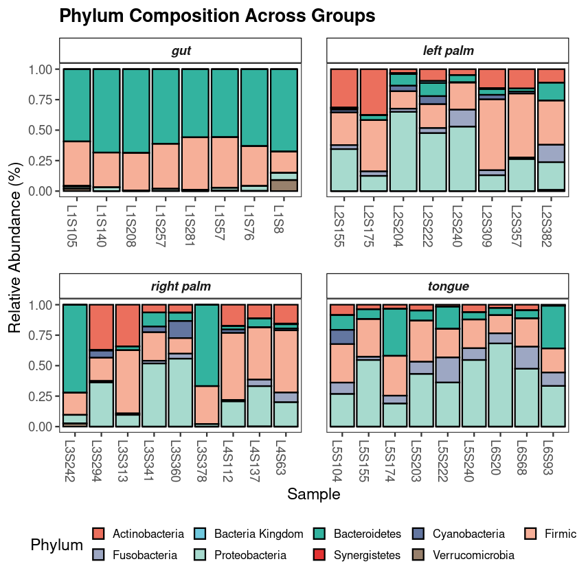
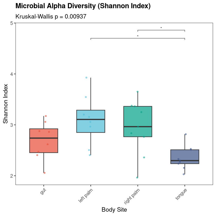
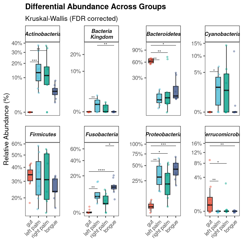
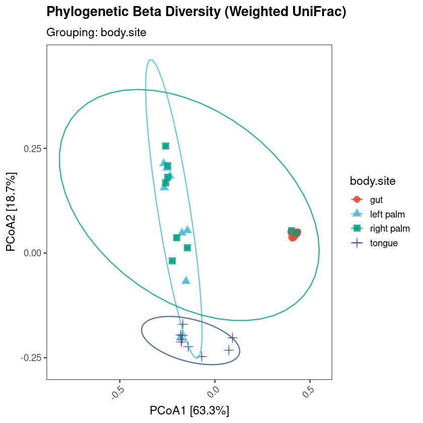
Get a ready-to-use 16S R code workflow and complete 16S pipeline for NGS meta-barcoding data downstream analysis and visualization in R. The script generates analysis-ready figures, exported CSV files, and a Methods section for microbiome projects.
Instant download. Individual license. No subscription.
This is a downstream analysis tool. It does not perform sequencing, denoising, or DADA2 processing. It starts where QIIME2 ends — with your preprocessed feature table — and runs the statistical analyses you need to interpret your data and write your Methods section.
You have processed 16S data (OTU/ASV table + taxonomy + metadata) from QIIME2, DADA2, or similar. You work in R. You want alpha diversity, beta diversity, differential abundance, and correlation analyses with analysis-ready ggplot figures and FDR-corrected statistics.
You need raw sequence fastq processing (DADA2, denoising, OTU picking).
Import directly from QIIME2 .qza artifacts (recommended) or from plain CSV/TSV tables if you have already exported your data.
Set your working directory path, your sample ID column, and your grouping variable. Everything else in the script derives from those three values.
13 labeled sections in RStudio. From taxonomic profiling to alpha/beta diversity, to differential abundance. Run them sequentially and start exploring your dataset and gaining biological insights in minutes.
Running all 13 sections generates the following outputs. The exact figure count varies slightly depending on your number of groups and whether a phylogenetic tree is available.
Phylum-level composition by group
Alpha diversity — Shannon + Observed
Differential abundance — top genera
Beta diversity — PCoA (Weighted UniFrac)
Taxa–metadata correlation heatmap
Each section is clearly labeled in the script. Run them in order in RStudio. The rarefied phyloseq object built in Section 2 is used by all downstream sections, so do not skip it.
Auto-installs missing packages from CRAN, Bioconductor, GitHub. Run once.
Set 3 variables. Choose QZA auto, QZA manual fallback, or CSV import.
Taxonomy cleaning, prevalence filter (5%), read depth histogram.
Rarefaction curves, depth selection at 90% of minimum, rarefied object.
Stacked bar chart + boxplots for top 8 phyla by group.
Top 4 phyla with auto-switching Wilcoxon / Kruskal-Wallis significance stars.
Top 4 genera with significance annotations and prefix cleaning.
Dominant taxa, group-level abundances, fast Spearman correlation preview.
Shannon + Observed, Kruskal-Wallis global test, Dunn post-hoc with FDR.
Jaccard NMDS, PERMANOVA (999 permutations), betadisper, taxa loadings plot.
Full PERMANOVA output table, betadisper visualization, TukeyHSD if needed.
Weighted UniFrac, PCoA with % variance explained. Requires phylogenetic tree.
Per-genus Wilcoxon or Kruskal-Wallis, Dunn post-hoc, FDR correction, forest plot.
Univariate models per genus, odds ratios + CI, train/test ROC curve, AUC.
CLR transform, Spearman × numeric metadata, global FDR, ComplexHeatmap.
Each section uses objects from the previous one. Run in order, check output, proceed.
# ── The 3 variables to set before running ───────────────────────────────── MY_WORKING_DIR <- "path/to/your/project/folder" MY_SAMPLE_ID <- "sample_name" # column identifying each sample MY_GROUP_VAR <- "Treatment" # your grouping column # ── Then choose ONE import option ───────────────────────────────────────── # Option 1 (recommended): QIIME2 .qza artifacts QZA_TABLE <- "table.qza" QZA_TREE <- "rooted-tree.qza" QZA_TAX <- "taxonomy.qza" QZA_METADATA <- "metadata.tsv" # Option 3: plain CSV tables (no tree → UniFrac section is skipped) CSV_OTU <- "your_ASV_table.csv" CSV_TAX <- "your_taxonomy.csv" CSV_METADATA <- "your_metadata.csv"
Package installation is handled by the script on first run. You need R, an internet connection for that first run, and your preprocessed data.
Direct link with immediate access after purchase.
microbiome-phyloseq-workflow.rStatistical_Methods_Summary.txtStatistical_Software_and_Bioinformatics_Packages.txtmicrobiome_workflow.pdfREADME.txtLicense.txtFor one researcher
For a research group or lab
No. This script starts after preprocessing. You need a feature table (OTU/ASV), taxonomy assignments, and sample metadata. Raw reads, DADA2, and denoising are not involved.
Run Section 1 of the script. It checks for each package and installs only the ones that are missing, from CRAN, Bioconductor, and GitHub. You do not need to install anything manually first.
Use Option 2 (manual QZA import) or Option 3 (CSV import) instead. Both are included in the script. Option 3 does not require qiime2R at all and works with plain CSV tables exported from any preprocessing tool.
Yes. Set MY_WORKING_DIR, MY_SAMPLE_ID, and MY_GROUP_VAR to match your project, then point the import section to your own files. The rest of the script runs on whatever phyloseq object is built from your data. Not every section will produce output for every dataset — for example, the correlation heatmap requires numeric metadata columns.
One person per purchase. You can use the script for your own research, adapt it for your own datasets, and cite it in your Methods section. You cannot share, redistribute, or republish the script — including in courses, tutorials, or shared lab repositories. Each user needs their own license.
Basic R familiarity is needed — you should be able to run code blocks, read error messages, and change variable values. The script is commented throughout, but it is a real analytical script, not a step-by-step tutorial. If you are new to R, expect to spend time on the initial setup.
No. The download is available immediately after purchase. Please read this page carefully and make sure the script matches your use case before buying.
Run it on your own dataset. Save days of coding & start gaining biological insights in minutes
Reach out via our Contact Form. We're here to help.